Simitar created this tool that it calls an ROI-Loading graph, or “ROIL” graph, and was invited to show it in the 2011 Winter Simulation Conference—the premier international conference for system simulation.  The tool displays results of multiple dynamic capacity analyses on a single graph.  Managers and engineers carrying this tool will have capacity answers always available.

Here is a graphic with instructions on how to construct the tool:

The full paper on this method follows.

Abstract

This paper describes a method for using Monte-Carlo simulation to estimate the profit-maximizing loading for each machine in a factory.  Multiple runs of a factory simulation model are made—with varying machine quantities—with the results graphically displayed as a correlation between static % loading and ROI (return on investment) for each machine purchase option.  The ROI is calculated from the estimated dollar value of the cycle-time reduction expected from that machine purchase and the purchase cost of the machine.  Management can thus graphically see the ROI for machine-purchase options for a variety of machines and compare them.  Such ROI-loading graphs—or “ROIL” graphs—once created, enable static models to benefit from past simulation runs: users graphically see the target static % loading of each machine type and also see how it will change if the budget or the required ROI change in the future.

1        OVERVIEW OF THE TRADITIONAL METHOD: STATIC-CAPACITY ANALYSIS VIA SPREADSHEET

The most basic way to model capacity is via a static spreadsheet.  A static spreadsheet takes into account machine quantity, machine downtime, number of visits per product type, processing time per visit, and other factors to produce a static % loading for each machine type.  When such a spreadsheet predicts that a machine type will be loaded more than a certain percentage in the future, action is  taken—such as ordering an additional machine—to reduce loading back below this number.

1.1         Shortcomings of Static-Capacity Analysis

Static capacity analysis’s major shortcoming is that it does not capture the effect of variability, which can be very high in some operations, such as wafer fabs.  Wafer fabs often must run at the very edge of technological capability to produce products which the market demands.  Machines thus pressed to the limit often suffer high downtimes and high rework and scrap rates.  Furthermore, in wafer fabs, machines are often visited many times by the same wafer—even approaching 100 visits—meaning that a neat production-line layout is not possible.  As a result, wafers must be regularly transported around the fab, incurring variable delays.  In many fabs, the machines are also used concurrently by R&D.  Combine this with up to 1500 operations required per completed wafer, and many product types running in the same factory, and you have more variability than with just about any other type of manufacturing operation.

Any operation with such high variability, if it were run at near 100% loading, would see exorbitant cycle times.  And low cycle time is especially important to fabs running R&D on the same machines because quick cycle time speeds up R&D learning cycles, meaning new products get developed and into the market more quickly, while price premiums are at their highest.  Mature products also gain an advantage from quick cycle times, given that technological advancement is reducing their market value daily.   Furthermore, short cycle times enable agile response to changes in customer demand.

Because of the variability inherent in wafer fabrication, and the high cost of cycle time, a fab typically sets its maximum allowable loading at some level well below 100%–65-85% is typical.  This is considered to provide the most profitable tradeoff between the cost of equipment and the cost of cycle time.  In choosing its maximum static % loading then, a company is choosing a de facto maximum acceptable cycle time.  The capacity of a fab, given such a self-imposed “ceiling” on cycle time, has been coined “cycle-time-constrained capacity” (Fowler and Robinson 1995).  This is the capacity of a fab, given that it will not accept a cycle time higher than a certain value.

So, if a fab’s maximum allowed static % loading is, say, 80%, a machine type that is forecast to be loaded 81%+  in the future would have that mitigated by a machine purchase or other action, whereas a machine type forecast to be loaded 80% or less would be left as-is.  But here we come to a major shortcoming of static capacity analysis:

Relative to static % loading, not all machines contribute to cycle time equally.

Furthermore:

Not all machines cost the same.

A simulation analysis could enable you to identify those machines that contribute the most to cycle time relative to static load.  Adding machine cost into this equation enables you to calculate a  cycle-time reduction per dollar for every machine-purchase option (Grewal et al [1998]).  Focusing your spending on your purchase options that produce the greatest cycle-time reduction per dollar enables you to achieve your cycle-time goal at lower cost—perhaps millions of dollars lower cost.

For example, let’s say that your static model projects that, in a future quarter, Machine A will be loaded 90% and Machine B will be loaded 70%.  Using a traditional straight-across 80% cutoff, you would buy another Machine A and not buy another Machine B.  But in reality, buying a Machine B may actually bring you greater cycle-time reduction than Machine A.  Why is this?

1.2         Some Factors That Cause a Machine’s Cycle-Time Contribution To Be High Relative to its Static % Loading

• High number of visits per wafer.  Take two identical machines with the same % loading and the same average queue time per visit.  But if one is visited once per wafer, and the other is visited fifty times by each wafer, the latter’s total queue time from this machine will be fifty times that of the first machine.
• Coarse machine granularity.  All else being equal, a single large-capacity machine will contribute more to queue time than a number of small-capacity machines.  For example, take two machine families, identical except that one consists of ten machines, each having a capacity of 50 wafers a day, and the second consists of a single machine, having a capacity of 500 wafers a day.  For the latter machine, capacity toggles between 100% and 0% as the machine goes up and down, creating queue-time spikes followed by lost production.   The ten small-capacity machines, on the other hand, won’t see such drastic change in capacity and will provide a smoother flow of product to downstream machines, resulting in shorter average queue times.
• Batch machine.  All else being equal, a batch machine has higher queue time relative to % loading than a single-wafer processor.
• Greater variability in downtime.  Take two identical machines with identical downtime percentages, the only difference being that the second machine fails less frequently but for longer periods of time.  The second machine will have longer average queue time than the first.

1.3         Enter The Simulation Model

A simulation model can take into account the above soup of factors and others and tell us the correlation between static % loading and resulting cycle-time reduction for each machine-purchase option.  At Simitar we realized that we could dollarize the benefit of this cycle-time reduction and compare it to machine cost to calculate an ROI  (return on investment) for each machine-purchase option.  Graph all of these machine-purchase options, and you have what Simitar calls a ROIL graph.

2        THE ROIL GRAPH

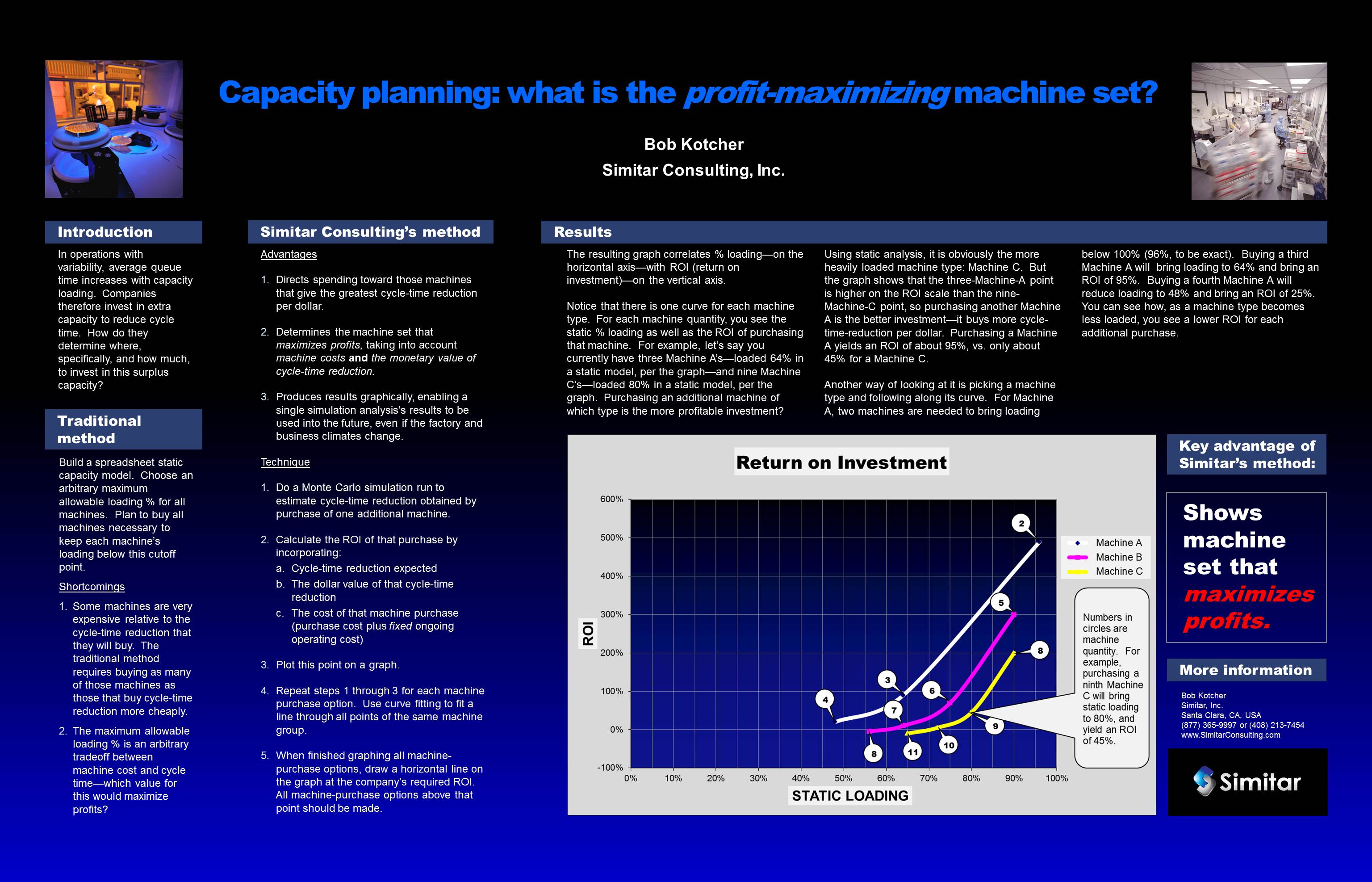
Figure 1 shows a ROIL (Return On Investment-Loading)  graph created with a simulation model.  You’ll notice that the ROIL graph correlates % loading—on the horizontal axis—with ROI (return on investment)—on the vertical axis.  This is simply a standard “operating curve”—which correlates % loading with queue time—but with queue time dollarized  and combined with the purchase cost of the machine to enable replacement of queue time with ROI.  Details on how that is done is described in section 2.1.

Notice that there is one curve for each machine type.  At a particular current % loading, the indicated ROI is what you’re likely to see if you purchase an additional machine of that type.  For example, let’s say you currently have three Machine A’s—loaded 64% in a static model, per the Figure-1 graph—and nine Machine C’s—loaded 80% in a static model, per Figure 1.  Purchasing an additional machine of which type is the more profitable investment?  Using static analysis, it is obviously the more heavily loaded machine type: Machine C.  But the ROIL graph shows that the three-Machine-A point is higher on the ROI scale than the nine-Machine-C point, so purchasing another Machine A is the better investment—it buys more cycle-time-reduction per dollar.  Purchasing a Machine A yields an ROI of about 95%, vs. only about 45% for a Machine C.

Figure 1: the ROIL graph shows the expected return on investment for each machine-purchase option

Another way of looking at it is by following along one curve.  For Machine A, if you have just two machines, the ROIL graph shows that they’re loaded 96%, and purchasing an additional one yields an ROI of 490%.  If you have three Machine A’s, the ROIL graph shows that they’re loaded 64%, and buying an additional one yields an ROI of 95%.  If you have four Machine A’s, loading is 48% and the ROI of purchasing an additional machine is 25%.  You can see how, as a machine type becomes less loaded, you see a lower ROI for each additional purchase.

2.1         Creating a ROIL Graph

Ranking purchase options by cycle-time-reduction-per-dollar is not new.  Creation of a ROIL graph takes this further by (1) incorporating the dollarized value of cycle-time improvement which, when combined with machine purchase cost, enables calculation of ROI, (2) graphically showing the result of multiple machine-purchase options, and (3) showing how the profit-maximizing machine set will change if the budget or required ROI change.

References

Chance, F., Carr, S., and Beller, K., 2001. What is One Day of Cycle Time Reduction Worth? FabTime Cycle Time Management Newsletter, Volume 2, Number 6, 3-6.
Chance, F., and Robinson, J. K., 2002. FabTime Bottom Line Cycle Time Benefits Calculator. Available at <http://www.fabtime.com/bottomline.shtml>[accessed April 29th, 2008]
Fowler, J. W., Robinson, J. K., 1995. Measurement and Improvement of Manufacturing Capacity (MIMAC) Designed Experiment Report, SEMATECH Technology Transfer #95062860A-TR.
Grewal, N. S., Brusky, A. C., Wulf, T. M., Robinson, J. K., 1998. Integrating targeted cycle-time reduction into the capital planning process. Proceedings of the 1998 Winter Simulation Conference, available at <http://www.informs-sim.org/wsc98papers/136.PDF>
Leachman, R. C., 2008. Methods of manufacturing improvement. Available at <http://www.ieor.berkeley.edu/~ieor130/cycle_time_notes.pdf> [Accessed April 29th, 2008]
Robinson, J. K., and Chance, F., 2002. The Bottom-Line Benefits of Cycle Time Management. FabTime Cycle Time Management Newsletter, Volume 3, Number 5, 7-10.
Robinson, J. K.. and Chance, F., 2006. Financial Justification for CT Improvement Efforts. FabTime Cycle Time Management Newsletter, Volume 7, Number 7, 4-8.
Author Biography
ROBERT KOTCHER is President of Simitar, Inc., an operations-improvement consulting firm based in Silicon Valley. He received his MBA from Santa Clara University and his BS in Industrial and Systems Engineering from San Jose State University. His career has covered simulation modeling, process improvement incorporating lean Six Sigma methods, and manufacturing engineering. He has previously presented papers on capacity planning and simulation modeling at the Winter Simulation Conference and at the International Symposium on Semiconductor Manufacturing. He is an ASQ Six-Sigma Green Belt and member of the Institute of Industrial Engineers.